IML Lab1 report
Author: Ruixuan Huang Student ID: PB20111686
Aims
- Implement logistic regression framework using given dataset
- Use the given dataset to test the model we trained
- Illustrate loss curve of one training process
- Give comparation table of different parameters
- Give the best accuracy of test data
Methods
Step1. Data process
The original dataset (loan.csv) is typical for dichotomous classification problem. Before using it to train models, I noted that there are some cases with missing attributes. Here my choice is using df.dropna() to discard these cases.
Then, we should convert non numerical descriptions of some attributes to continuous numerical descriptions. I noted that the values of each to-be-converted attribute have some order relationship. So I simply use df[{attr_name}].map() to convert.
In addition, I normalized the variables (except Loan_Status). This is because I noticed that the numeric accuracy of Python is also to be considered. Some values of orginal data is so big that the sigmoid function will directly give the output 1.0 during every iteration. Thus \boldsymbol\beta could not update.
I decided to use hold-out method to train a model. So my strategy to split the dataset can be described as follows:
- Use
df.sample(frac=1.0)to randomize the dataset - Use
df.sort_values("Loan_Status", inplace=True)to place the positive and negative cases in two consecutive areas to facilitate the data spliting - In the positive area, choose its top 40% cases and add them into
X_trainandy_train. For negative cases the rate is 80%. This is because the proportion of positive and negative of original dataset is 2:1 - After executing the above 3 procedures, I get the
X_train,X_test,y_train,y_test
Step2. Implement the LR class
According to the (3.27) in the textbook, our objective is to minimize
I assumed that fit_intercept=True, so here \boldsymbol{\beta}=(\boldsymbol{w};b),\hat{\boldsymbol{x}}=(\boldsymbol{x};1).
In my code I also dealt with the situation when
fit_intercept=False, but in the report I'll only discuss the situation whenfit_intercept=True.
I use \displaystyle\sigma(x)=\frac{1}{1+e^{-z}} as the sigmoid function, so the result of one prediction is \sigma(\boldsymbol{\beta}^\top\hat{\boldsymbol{x}}).
Now implement the training (fit) method. The cost function is
I use gradient descent to decrease the cost function and find the optimal \boldsymbol\beta. According to the (3.30), the gradient function is
In each iteration, if the absolute value of the increment of the cost function is less than the parameter tol, the iteration will break, which means the training is done. Otherwise the \boldsymbol\beta should update according to
Here \alpha is the parameter lr. The training has a maximum number of iteration which is set by the parameter max_iter. One more thing, in order to draw a loss curve, the fit method will return an array of values of cost function during the training process.
The last thing is implementation of predict method. It will use the trained \boldsymbol\beta to caculate a result for each line in X_test. The result will be caculated according to
And the predict method will return an array of results from all test lines.
Step3. Train and test in framework
Now I have the split dataset (X_train, X_test, y_train, y_test) and LR class. Simply call the fit method on X_train and y_train. And using matplotlib to illustrate the loss curve according to the return value of fit.
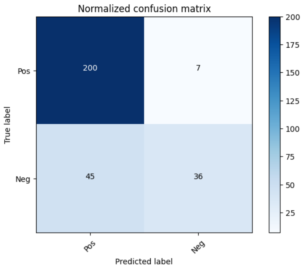
In the test process simply call the predict method on X_test and get its return value. Then compare each element of it and its corresponding label in y_test. In this process I will use a confusion matrix to display the result of the trained model running on the test dataset.
Step4. Using different parameters
In order to get the comparation table, I repeat the steps above using one different parameter each time, using accuracy \left(\displaystyle\frac{TP+FN}{TP+TN+FP+FN}\right) as the metric. For lr, there will be a extra metric: trend of the loss curve.
Result
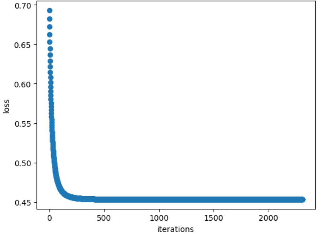
Loss curve
The loss curve (one training process) of training process is as follows. Here the y-axis represents the value of cost function, the x-axis represents the number of iterations.
Comparation table
The original parameters I picked is:
- Positive and negative cases ratio in test dataset (PNR): 1:1
- Ratio of training set data to all (TAR): 50%
- Learning rate (lr): 0.1
- Penalty and gamma: \gamma=0.01,L1
Define some varibles as follows:
mark meaning c_0 the number of negative cases of the dataset c_1 the number of positive cases of the dataset t_0 the number of negative cases of X_train t_1 the number of positive cases of X_train The four variables above satisfy the following formulas: $$ TAR=\frac{t_0+t_1}{c_0+c_1}\quad\quad PNR=\frac{t_1}{t_0} $$ Given certain TAR and PNR, we can get $$ t_0=\frac{TAR\times(c_0+c_1)}{1+PNR}\quad\quad t_1=PNR\times t_0 $$ The results above make it easier to change the parameter TAR and PNR when watching their effect of training, which enables us to be free of caculating the size of training set. But one thing to be noticed is that $$ \textbf{assert } t_1 <= c_1\textbf{ and }t_0 <= c_0 $$
Then each time I will use one difference parameter on the basis of these values.
PNR
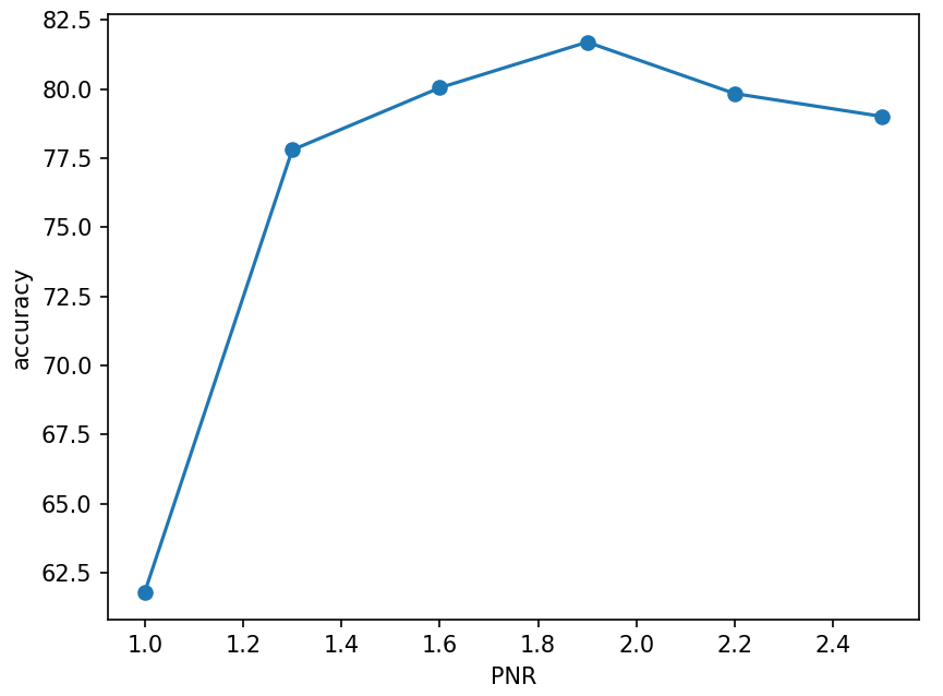
| PNR | 1:1 | 1.3:1 | 1.6:1 | 1.9:1 | 2.2:1 | 2.5:1 |
|---|---|---|---|---|---|---|
| Accuracy | 61.79% | 77.79% | 80.04% | 81.69% | 79.83% | 79.00% |
- Other: TAR=0.5,lr=0.1,tol=10^{-5},\gamma=0.01,L1
- Each PNR case repeated 10 times, The result is the average.
TAR
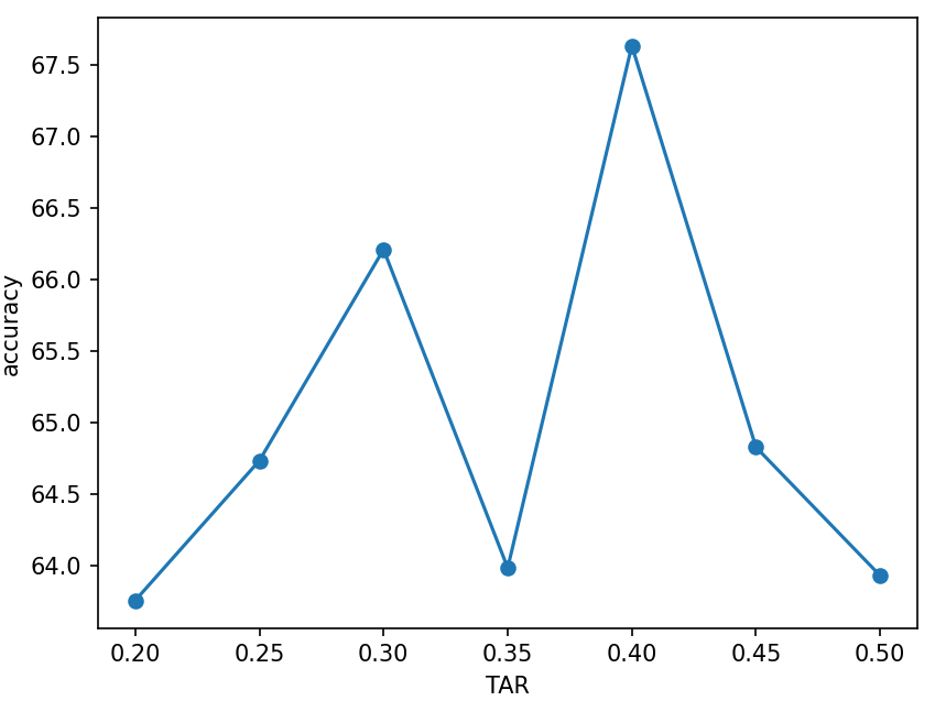
| TAR | 20% | 25% | 30% | 35% | 40% | 45% | 50% |
|---|---|---|---|---|---|---|---|
| Accuracy | 63.76% | 64.74% | 66.21% | 63.99% | 67.63% | 64.82% | 63.93% |
- Other: PNR=1:1,lr=0.1,tol=10^{-5},\gamma=0.01,L1
- Each TAR case repeated 10 times, The result is the average.
lr
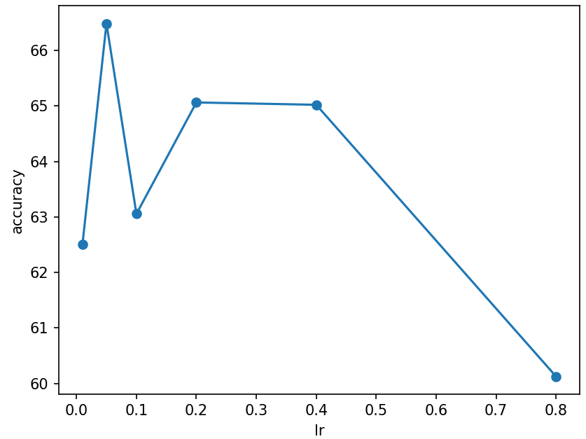
| lr | 0.01 | 0.05 | 0.1 | 0.2 | 0.4 | 0.8 |
|---|---|---|---|---|---|---|
| Accuracy | 62.51% | 66.48% | 63.05% | 65.06% | 65.02% | 60.12% |
- Other: PNR=1:1,TAR=50\%,tol=10^{-5},\gamma=0.01,L1
- Each lr case repeated 10 times, The result is the average.
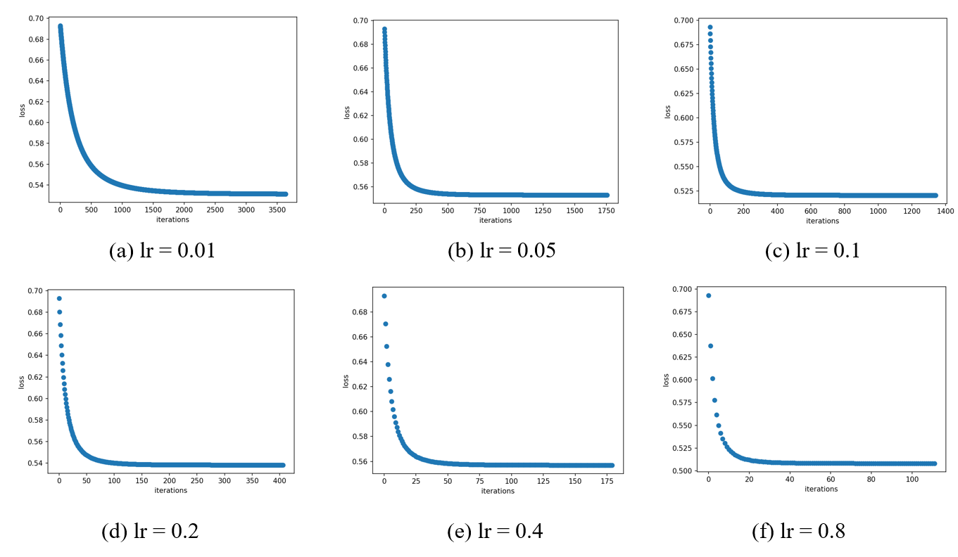
The loss curve for each case of lr. We can intuitively conclude that the larger the value of lr, the faster the loss function decreases.
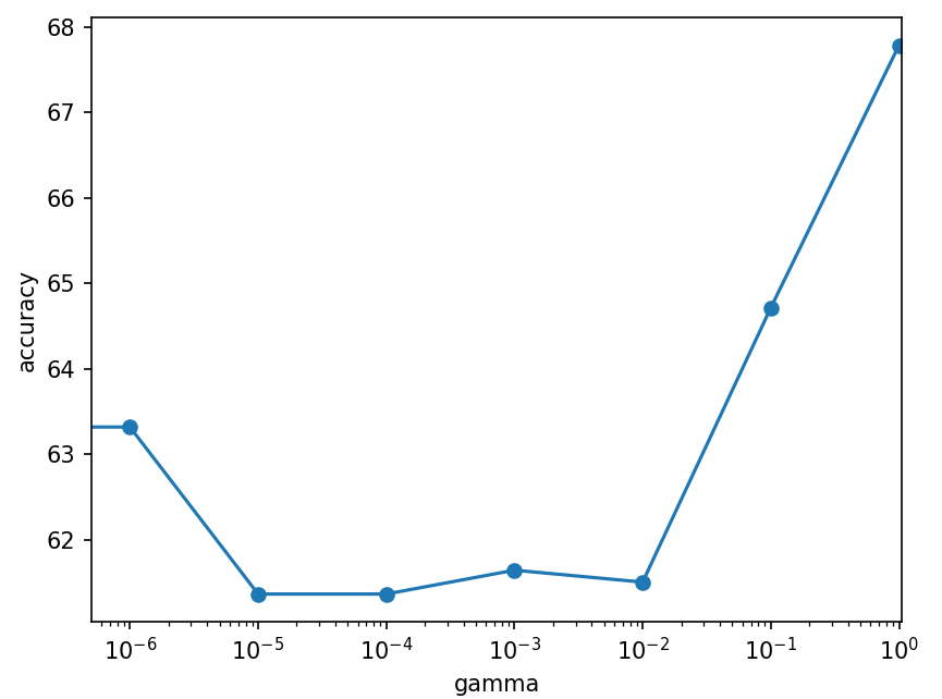
penalty and gamma
penalty = "L1"
penalty = "L2"
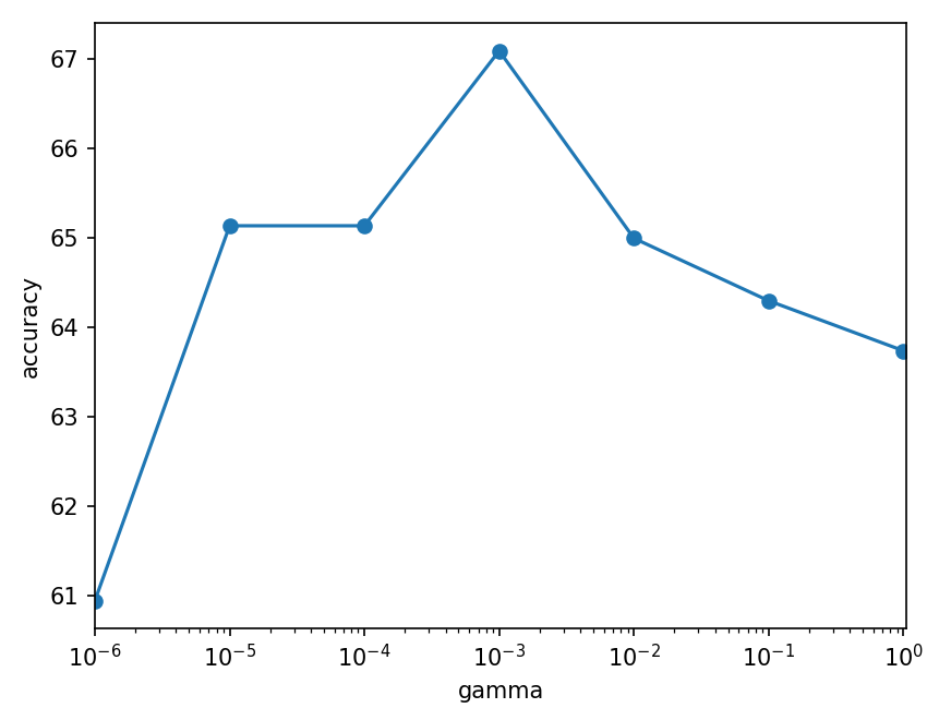
| gamma | 1 | 1e-1 | 1e-2 | 1e-3 | 1e-4 | 1e-5 | 1e-6 | 0 |
|---|---|---|---|---|---|---|---|---|
| L1 | 67.78% | 64.71% | 61.50% | 61.64% | 61.36% | 61.36% | 63.31% | 64.43% |
| L2 | 63.73% | 64.30% | 64.99% | 67.08% | 65.13% | 65.13% | 64.29% |
- Other: PNR=1:1,TAR=50\%,tol=10^{-5},lr=0.1
- Each lr case repeated 3 times, The result is the average.
Best accuracy
From the results above, the best accuracy is 81.94%, which has these parameters: $$ PNR=1.9:1\quad TAR=0.4\quad lr=0.05\quad tol=10^{-5}\quad penalty=L2\quad \gamma=10^{-3} $$ Its confusion matrix is